Mark Fackrell on Distributions

Nosokinetics

Phase-type Distributions in Healthcare Modelling I

by Mark Fackrell (Editor's Summary)

Necessity is the mother of invention. Mathematics is a high level language, with many symbols expressing concepts. Till now we have scanned formulae, however, given the quality of Mark's article and the promise of two more, we have created a Tutorial section on the Nosokinetics website at www.nosokinetics.org.

This article first explains why stochastic(random) models are needed. One compelling reason is that performance measures need to be determined, so sensible decisions can be made. Another is that stochastic models often perform better than deterministic models, because randomness underlies many real world systems.

Probability theory relies on the concept of a random variable. Consider tossing a coin. The experiment may be tossing three fair coins, and the random variable is the "number of heads". Associated with any random variable is a distribution function. In this example the probability of tossing 0,1,or 2 heads is 7/8.

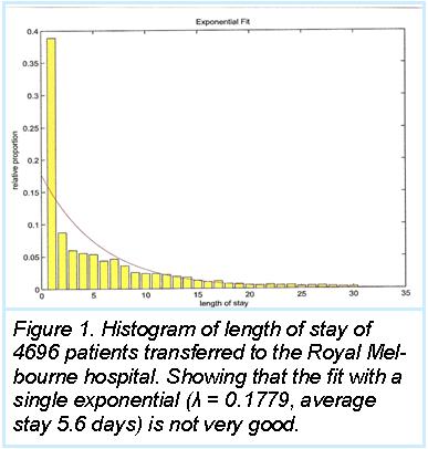
Discrete random variables have discrete values e.g. 0,1,2 and 3. Whereas, continuous random variables take values from an interval e.g. the "length of stay in an emergency department". One very important continuous distribution is the exponential distribution, which has the unique feature of being memoryless.

Figure 1 shows that the fit between a single exponential and length of stay of transferred patients is not very good. So better stochastic models are needed. Here is where phase type models come into the picture. Here we need the concept of a (finite state) continuous time Markov chain.

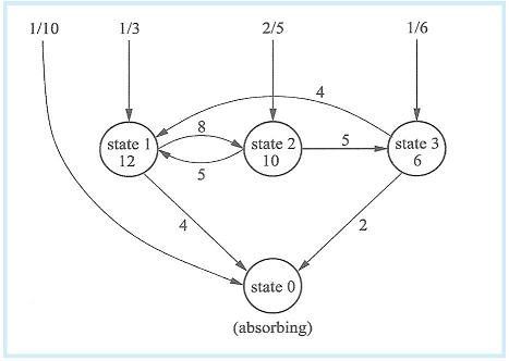
In Figure 2 the state space S = {0,1,2,3} and we select a state according to the initial state probability vector = (1/10, 1/3, 2/5, 1/6). Once in each state we spend an exponentially distributed time lamda in each state (for example lamda = 12 for state 1) and then move to another state with a certain rate. We go from state 1 to state 2 with rate 8, and from state 1 to state 0 (the absorbing state ) with rate 4. So rate 12 can be thought of as the rate "out" of state 1. The process continues until we end up in state 0 where we stop.

Read the full text in a pdf version.

[To Contents Page] [To Archive Overview]

Some navigational notes:

A highlighted number may bring up a footnote or a reference. A highlighted word hotlinks to another document (chapter, appendix, table of contents, whatever). In general, if you click on the 'Back' button it will bring to to the point of departure in the document from which you came.